Tutorial for Students

Example Problem Setup and Solution Using Cyclepad

The Problem:

Let's say we want to do a problem like the ones given for homework. For our example we will do problem 9.23 (VanWylen et al, 4^th edition). The problem statement is:

Consider an ideal steam combined reheat and regenerative cycle in which steam enters the high pressure turbine at 3.5 MPa, 400ºC, and is extracted for feedwater heating at 0.8 MPa. The remainder of the steam is reheated to 400ºC at this pressure, 0.8 MPa, and is fed to a low-pressure turbine at 0.2 MPa for feedwater heating. The condenser pressure is 10 kPa. Both feedwater heaters are open heaters. Calculate the thermal efficiency and the net work per kilogram of steam.

What it looks like:

The problem describes a system that looks like the following:

Overview:

We will solve this problem using Cyclepad. Cyclepad allows us to build, analyze, and alter a thermodynamic cycle design, often far more easily than is possible to do by hand. Once we are proficient in setting up a cycle in Cyclepad, we can solve many basic cycle problems in only a few minutes. More importantly, Cyclepad allows us to change designs easily, either by changing numerical values (what happens if the pressure in the condenser were 50 kPa instead of 10 kPa?) or by adding or removing components in the design (what if there were only one feedwater heater?). In addition, Cyclepad's Sensitivity Analysis tool allows us to see how various cycle parameters change as we change certain values over a range, allowing us to see plots of things like the thermal efficiency of the cycle as we change, for instance, the boiler pressure from 3 MPa to 4 MPa.

As we go through this example, we will see how Cyclepad helps solve design problems by doing calculations and looking up table values for us. We will also see how our own knowledge of thermodynamics is key to telling Cyclepad how to go about solving a cycle.

Starting Cyclepad:

When we open Cyclepad, we see the Open New Design dialog, where we tell Cyclepad the title of our design, whether it is an open (steady-state, steady-flow) cycle or a closed (control mass) cycle, and whether we want Cyclepad to calculate efficiencies for a heat engine, heat pump, or a refrigeration cycle.

Let's title our problem "Problem 9-23" and tell Cyclepad we are dealing with an open cycle heat engine. Then click OK.

Adding devices to the design:

After the Open New Design dialog disappears, Cyclepad shows us the Device Palette. The Device Palette contains the following devices:

heater cooler heat exchanger
pump compressor turbine
throttle splitter mixer
source reactor sink

To add a device to our design, we click on the device on the Device Palette, then click on the spot on the design where we want that device to be. Devices can be moved by dragging, and right-clicking on a device brings up a menu allowing us to change its orientation or delete it.

Our first task, then, is to add all of the devices we will need to our design. Let's start with the heater and work our way clockwise around the schematic above. After the heater, we place the high-pressure turbine. We notice that, before we reheat the fluid that leaves the high-pressure turbine, some of it splits off and goes down to mix with other fluid (feedwater heating). To allow for this fluid to split off, we add a splitter. The picture at the left shows what we have so far.

Looking at our schematic, we see that the next component is another heater used to reheat the fluid before it enters the low-pressure turbine. So, we add another heater in Cyclepad.

Now we notice that the low-pressure turbine has two stages. One that goes from 0.8 MPa to 0.2 MPa, and a second that goes from 0.2 MPa down to 10 kPa. In between these two stages, some more fluid is split off and sent to a second feedwater heater. Each Cyclepad turbine has just one inlet and one outlet, so we will draw the two-stage low-pressure turbine as two single-stage turbines with a splitter in between them.

The rest of the design can be added pretty much just as it appears in our schematic. After the turbines, we add a cooler. Then we finish with a sequence of three pumps separated by two mixers. This completes the addition of all necessary components to the design. As a quick bit of aesthetic tweaking, we can right-click on HTR2 and rotate it 90  clockwise so that its inlet and outlet arrows point the right way. At this point, our design is:

Our final build task is to connect all of the inlets and outlets of our components. We notice that whenever we click on an inlet or outlet, Cyclepad highlights in red all of the inlets or outlets to which we might connect. We can make the connections in any order. In this example, we made the connections starting after the first heater, then proceeding clockwise around the components, connecting the splitters to the mixers last. Cyclepad numbers the statepoint between each connection as it is made. Our fully-connected design looks similar to the one shown below.

After all inlets and outlets are connected, Cyclepad, tells us that we have a complete design and asks if we wish to switch to Analyze Mode, which is what we want right now. If we wanted to stay in Build Mode, we could add and delete more components, change the label names, or move things around to suit our tastes better.

Analyzing our design:

When we switch to Analyze Mode, Cyclepad takes a few minutes and tries to solve many of the equations which apply to our design. Many more equations will be added as we tell Cyclepad which assumptions apply to the various components. When the hourglass goes away, we can start making assumptions about the devices in our design and the statepoints connecting them. For this example, we will go around the design and add what information we know as we go, clicking on each device or statepoint to get its meter window to show up. It is particularly during this stage that our own knowledge of thermodynamics is critical to making assumptions Cyclepad will use in design solution. We start at the heater.

HTR1: When we open up a meter window, it shows everything we know about a statepoint or device. The things we know because we have assumed them are shown in green. The things we know because Cyclepad has figured them out are shown in blue. The things we do not know are shown in black. Since we initially know nothing about the heater, everything is shown in black.

We aren't explicitly told anything about the heater, but we know that ideal heaters are generally considered to incur no pressure loss. Click where the words Make Assumption appear to allow Cyclepad to show us the assumptions available for a heater. We see that there are essentially two assumptions: that the heater is or is not isochoric (zero change in specific volume) and that the heater is or is not isobaric (zero pressure change). Click on HTR1 works isobarically to assume that our heater has no pressure change.

We notice that Cyclepad shows our assumption in green and that it also now shows a second modeling assumption (that the heater is not ISOCHORIC) that Cyclepad has figured out based on our assumption and its own background knowledge (that a heater cannot be both isochoric and isobaric). The rest of the entries in the heater window remain black since nothing is known about them yet. To see what each of the symbols on the left stands for, click on it (holding down the mouse button) and its English name will pop up.

S1: Looking now at the statepoint after the heater, we know both the pressure and temperature of the fluid at this statepoint from the problem statement. Click on the blue bulge representing that statepoint and its meter window will pop up. The first thing we know about this statepoint is that our working fluid is made of water (steam). Clicking on the word UNKNOWN next to Substance, then we can choose to pick a substance. On the list of substances shat show up, water is at the bottom. We choose it and notice that the meter window has changed to allow more properties. (We may have to scroll down or make the meter window larger to see them.) Since water is a substance for which we have table values (instead of being an ideal gas), we see values for saturation properties as well as the other properties.

We also know the temperature and pressure at this statepoint. Clicking on the UNKNOWN next to T, we can assume a value for the temperature at this statepoint. Type in 400, since the units are already given as Celsius degrees. (If we needed to change them, we could go to "design" under the "Preferences" menu.) We do the same thing to assume the pressure value at this statepoint is 3.5 MPa (entered as 3500 kPa, since the units are in kPa for the entry window).

When T and P have been entered, Cyclepad pauses for a second and figures out the other intensive properties at this statepoint, like specific volume, specific internal energy, et cetera. If we were doing this problem by hand, these are all values we would have to look up in tables.

Let's stop for just a second and take a peak at the meter window for the statepoint just before the heater. Notice that the substance and pressure are already known. Cyclepad knows that there is only one fluid in this problem, so it must be the same one (water) we just assumed at S1. In addition, Cyclepad knows the pressure at this statepoint because we have told it there is no pressure change across the heater (we assumed it was isobaric), so it must be the same as at the statepoint after the heater. In this way, Cyclepad can save quite a bit of work in repeatedly entering values.

TUR1: Click on the first turbine to see its meter window. We aren't told anything explicitly about this turbine, but we are told it is ideal. In general, this means it is isentropic (zero change in entropy) and adiabatic (no heat transfer). Even if we did not know that it was ideal, we would probably assume it to be adiabatic because we have not been told how much heat transfer takes place and we have no way to figure it out. It is important that we know this and assume it in Cyclepad; it does not know it on its own. Clicking on Make Assumption, we assume TUR1 work adiabatically. Then click on Make Assumption again and assume TUR1 work isentropically.

We see again that Cyclepad determines some other things about the turbine as we give it more information.

S2: Click on the bulge after the turbine. Notice that the specific entropy is already known. (It is the same as that for the statepoint before the turbine because the turbine is isentropic.) We are told in the problem that steam is extracted from the high pressure turbine at 0.8 MPa, so we assume the pressure at this point to have that value. (Enter "800" because we are in kPa in the entry window.) Since Cyclepad now knows both the pressure and the entropy at this statepoint, it can figure out all of the intensive property values here. Once again, Cyclepad has saved us much time in table lookup, especially since this statepoint would require interpolation to find.

SPL1: We are told nothing about the splitter. Looking at its meter, we note that we could specify a splitting fraction for it, forcing a certain fraction of the entering fluid to leave through the down leg and the rest to go to TURB2. But we don't need to do that, since we want just enough fluid to split off so that that the fluid entering PMP3 is a saturated fluid. Cyclepad will figure out how much this is when we tell it what we want for S12.

S3: We already know everything about S3 since it is the same stuff that came out of TUR1.

HTR2: Once again, we have an ideal heater, so we assume that it is isobaric.

S4: We are told that the fluid is reheated to 400 C, so we can assume this temperature at the statepoint after HTR2.

Take a peek back at HTR2's meter window now. Notice that Cyclepad has figured out how much heat (q) is needed to heat the fluid from statepoint S3 to the values we specified at statepoint S4.

What if we had made a mistake in entering the temperature at S4? There are two things we can do. If we simply want to change a numerical value, click on the text of the current value, then choose Change the value of T(S4) and we can enter another value. If we want to take back an assumption entirely, we would choose Retract the value of T(S4), which also works for non-numerical assumptions (isentropic, isobaric, and so forth). In this case, 400 C is the temperature we want, so we can just enter that again.

TUR2: Once again, we assume this ideal turbine is adiabatic and isentropic.

S5: The problem specifies that the steam extracted for the second feedwater heater is at 0.2 MPa. So we can assume that pressure at this statepoint.

SPL2 and S6: Nothing to do here.

TUR3: As with turbines 1 and 2, we assume this ideal turbine is adiabatic and isentropic.

S7: The problem specifies that the condenser (cooler) pressure is 10 kPa. We assume this pressure at S7.

CLR1: Similar to an ideal heater, an ideal cooler has no pressure drop, so we make the isobaric assumption here as we did with HTR1 and HTR2.

S8: This is a statepoint when our own knowledge and reasoning about cycles is key to making assumptions. The only reason we have a cooler before the pump at all is because we know pumps can be damaged by non-liquids. To avoid this, the cooler must condense all of the steam leaving the turbine into a liquid before we send it to the pump. So we at least want to cool our saturated working fluid to 0% quality before sending it to the pump. Of course, pumps work fine with compressed liquids as well, so we could cool the fluid even past saturated fluid down into the compressed liquid region. We do not do this because we don't want to do any cooling that we don't need to (since we are essentially throwing away that heat). So, we try and cool just to saturated fluid, but no further.

For Cyclepad, we can specify the fluid at S8 to be a saturated fluid by going to Phase and selecting a phase and choosing it to be saturated. Once we have told Cyclepad that the phase is saturated, it adds another property to the meter window, allowing us to specify a quality. We assume values for quality as we do any other property (like we have for temperature and pressure). In this case, we want to assume that quality is zero, since we are forcing the fluid at S8 to be a saturated liquid.

PMP1: We are given no explicit information about the pumps, but, like the turbines, ideal pumps are adiabatic and isentropic. We assume both of those things here.

S9: The pump's purpose is to get the fluid coming out of the cooler up to a high enough pressure that we can mix it with the reheat steam coming out of the second turbine. If we make the pressure any less, the higher pressure of the reheat steam will force it back into the cooler, which is no good. If we make it higher, we will force fluid back through TUR2, which is also no good. So, we make the pressure at the pump outlet to be the same as that of the fluid.

How do we make these two pressures the same? Since we know this pressure is 200 kPa at S5, we could do it the way we have done before, clicking on UNKNOWN next to P and choosing Assume a value for P(S9), but there is a another way. What we really want to do is to make the pressure at S9 the same as the pressure leaving TUR2, whatever that pressure is. That way, if we decide to change the pressure at the turbine outlet (to see how it affects cycle efficiency, for instance), we won't have to change S9 again.

To do things this more flexible way, we choose Equate P(S9) to another parameter. This brings up the Equation Editor, which allows us to equate the parameters of any two statepoints or devices or whatever (Cyclepad calls these two things "entities"). Since we were looking at the pressure at S9, the parameter is already set to P and the entity is set to S9. The entity to which we wish to equate is S5 (the outlet of the second turbine), so we choose that from the pull down menu (as shown) and then click on Add so that Cyclepad can make the equation active. Once that is done, we can close the Equation Editor window and note that the pressure for statepoint S9 is 200 kPa.

MXR1: There is nothing special for us to do here. Looking at the meter for this device, we note that Cyclepad will compute the entropy increase due to the mixing, since mixing two dissimilar fluids that were separated increases the disorder in the world.

S10: As with state S8 we want to use the feedwater heating to heat the subcooled water up as much as we can so that it is no longer subcooled, but not so much that some of it evaporates and we have a non-liquid going into PMP2.

PMP2: We can assume our ideal pump here is adiabatic and isentropic, as PMP1 was.

S11: As with state S9, we want to equate the pressure of the fluid here to the pressure of the fluid we are mixing with it. Equate pressure at S11 with pressure at S2.

Notice that, down towards the bottom of PMP2's meter window, Cyclepad has figured out the shaft work per kg of fluid (the specific shaft work) needed to take the fluid at S10 to the pressure at S11. Normally we have to do this by hand and we still want to know how Cyclepad did it, so how do we check? Click on the number next to spec shaft-work and then click on the top item, Why does ... to bring up the Cyclepad Explanations dialog. This window explains how a number was gotten, usually by listing the equation used to calculate the number and the values of the known variables in the equation. Here we see that Cyclepad has used the equation w = – v DP.

Now, we know that reversable work is   , so now let's check how Cyclepad got from there to its equation by clicking on the equation, then clicking on Explain the rationale for spec shaft-work(PMP2) = -[v(S10*delta-P(PMP2)]. Text rationales are not available for all of Cyclepad's equations, but we can always use the Why is tool to track how Cyclepad got its numbers.

MXR2: Not much to interest us here.

S12: This statepoint is like S10; we want to heat the subcooled water going into PMP3 until it is a saturated liquid.

PMP3: We can assume this ideal pump here is adiabatic and isentropic, as were pumps PMP1 and PMP2.

We should note that, if we assume PMP3 to be isentropic before we assume it to be adiabatic, then sometimes Cyclepad finds a small heat transfer for the pump and, because this heat transfer isn't quite zero, Cyclepad asserts that the pump is not adiabatic or causes a contradiction when we assert that the pump is adiabatic. Why does this happen? The reason lays in the approximation that the water in the pump is incompressible, which is very close to accurate, but the slight variation in v between the saturated liquid at the inlet and the compressed liquid at the outlet causes this small heat transfer to show up, confusing Cyclepad. For our purposes, this heat transfer is not important (it is about 0.1% of the work done by the pump), so we can just not assume PMP3 is adiabatic if it causes a contradiction. In general, we might try to change the order in which we make assumptions, just to be certain no contradictions occur later on.

Finishing the problem:

Our original problem was to find the thermal efficiency of this cycle. Go to the "Global Properties" menu and choose "Whole Cycle." Here we see that the thermal efficiency is just over 38%.

However, we notice that Cyclepad still does not know the many of the values in this cycle. The reason is that Cyclepad finds some whole cycle properties based on extensive values (in other words, the whole heat transfer Q, not the specific heat transfer q). To see these values, assume a mass flow rate so that Cyclepad can compute the extensive values it needs to finish the whole cycle calculations. Go to state 1 and assume a mass flow rate of 1 kg/sec. Now, we see that those other properties are calculated.

While we're looking at the whole cycle properties, we might be curious how fast we need to run steam through this cycle to get, let's say, 100 kilowatts of power out of it. We can retract the value for m-dot from S1 and assume net-power in the cycle meter to be 100 kW. Then looking back at m-dot, we see we only need 0.09 kg/sec to get that much power from this cycle.

Now, 0.09 kg/sec certainly doesn't seem like a lot of water to generate 100 kW of power. But how much power is 100 kW really? In the Cycle meter window, click on the text of 100.0 kW and choose the last option, Show benchmarks for ... The graph that shows up gives us some feel for just how much power 100 kW represents and, it's really not that much. Cyclepad can show benchmarks for other properties as well, such as temperature and pressure.

Using the Sensitivity Tool:

What if we wanted to know how various parameters affect the cycle efficiency? For example, we notice that the pressure at the outlet of the third turbine is actually lower than atmospheric pressure; why is that? Well, we can use the Sensitivity tool to figure this out.

Go to the Tools menu and choose Sensitivity. This brings up the Sensitivity tool. With this tool, we can specify an independent parameter (the one we change, or x-axis) and a dependent parameter (the one we watch, or y-axis). For the example we are examining, the independent parameter is the pressure at the turbine outlet (S7) and the dependent parameter is the cycle's thermal efficiency. The cycle thermal efficiency is the default parameter the pops ups with the Sensitivity tool. To specify the turbine outlet pressure as the independent parameter, click on Stuff or Device under Independent Parameter and choose S7. Then, under Parameter to Vary, choose P. Now set the starting pressure to 0 kPa and the ending pressure to 200 kPa. Then click on Plot to start the tool working.

Looking at the resulting plot, we see that the outlet pressure has a considerable effect on h_thermal, changing it from 39% down to under 25% over the pressure range we specified. (We can also note that Cyclepad has trimmed off the data point at 0 kPa that would have given us an out-of-bounds error since we have no table data for water at absolute vacuum.) We can reason that the trend of the plot towards lower cycle efficiency with higher outlet pressure makes intuitive sense because the higher pressure represents energy in the fluid that we are not utilizing.

We could do sensitivity analyses for many other parameters as well. For instance, we assumed that the pressure at which we took steam for the second feedwater heater was 200 kPa. Though this number was given in the problem, we might guess that if we take it at a higher pressure, we might need less steam to heat the same water in the return path and we might then get a more efficient cycle. Doing a sensitivity analysis with the pressure at statepoint S5 would tell us if we are right.

Looking at the plot, we see that there actually appears to be a "best" efficiency point at around 140 kPa. To see the values of the points on a plot, move the mouse over a red data point and that point's value will appear in the lower left corner of the plot window. So, if we were actually looking to design a high efficiency plant, this is where we might want to extract our feedwater. Of course, it is important to keep the scale of the plots in mind; the whole range of h_thermal shown on this plot is less than 1%, so varying pressure at S5 may not be a big deal.

---

Problem 9.57

A stoichiometric mixture of gasoline and air has an energy release upon combustion of approximately 2800 kJ/kg of the mixture. To approximate an actual spark-ignition engine using such a mixture, consider and air-standard Otto cycle that has a head addition of 2800 kJ/kg of air, a compression ratio of 7, and a pressure and temperature at the beginning of the compression process of 90 kPa, 100 C. Assuming constant specific heat, determine:

(a) The maximum pressure and temperature of the cycle

(b) The thermal efficiency of the cycle

(c) The mean effective pressure

From the file menu choose new.

Name the design "Otto Cycle" and select closed.

Click OK.

The Otto cycle is composed of the following 4 stages: heating, expansion, exhaustion and compression. Build the cycle as depicted in the diagram below:

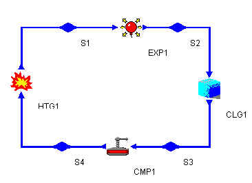
Click on each item on the component palate and then click on the blueprint region. If you right-click on an object you can rotate or delete it. To connect components, click the red arrow of the first component and then click the input arrow of the next component. This will link them.

When the cycle is complete, switch to analyze mode (if necessary, choose analyze from the Mode menu).

An Otto cycle has the following properties (as written on p382 of your text):
isentropic, adiabatic compression
isochoric heat addition
isentropic, adiabatic expansion
isochoric heat rejection (exhaust)

We also know that we can assume that the isentropic processes are adiabatic (no heat loss occurs) because ideal processes are reversable and any process which is reversable and isentropic must also be adiabatic.

For the heater, we know from the problem statement, that q=2800 kJ/kg. The compression ratio is given as 7. Click on the variable "r" in the compressor to see its full name. Enter the value 7.

Enter these assumptions for each device by clicking on the device.

Now enter the other information as specified in the problem above. Click on one of the stuffs (the blue diamonds). Choose air as the substance. Also enter the following information in the appropriate stuffs:
stuff entering compressor: 90 kPa, 100 C.

From the Global Properties menu, choose Whole Cycle. Record your answer to part a.

The maximum pressure and temperature of the cycle _______________________________

The system is still not calculating the efficiency or the mean effective pressure. Click on UNKNOWN% (next to eta-thermal) and select "How could I compute eta-thermal (CYCLE)" This will show you what pieces of data CyclePad is missing. You can continue to ask questions. Click Done when you have finished exploring.

There are two things which CyclePad needs to know to make the remaining computations: the mass and the work. You can assume a value of 1 for mass (enter this in any of the stuffs).

From the Global Properties menu, choose Whole Cycle. Record your answers to parts b & c.

The thermal efficiency of the cycle___________________________

The mean effective pressure________________________________

Compare your answers with those in the back of the book
a. 10.07 MPa; 4525 K
b. 0.541
c. 1957 kPa

You might notice a slight difference between the book answers and CyclePad's there are a few things you should know:
- You can change the units for one particular design by selecting Design from the Preferences menu. Click on the units tab. For example, you might want to change Temperature to Kelvin. You can also change the units for all your designs by choosing Global from the Preferences menu.
- CyclePad interpolates table values which might be different than yours
- CyclePad always assumes constant specific heats
- CyclePad sometimes assumes that a value which is "close" to another value actually is that other value.

---

Back to Software page | Back to QRG Home Page