CyclePad_Help

CyclePad has a fairly simple economic model that you can activate by choosing Preferences|Advanced and checking Consider Economics.  We describe the underlying model in this section.

The punchline of an economic analysis is the Net Present Value, or NPV, of the cycle you have created.  This is how much the cycle is worth to us today, given the interest rate at which we can invest our money and the amount of money we expect to make once we construct the cycle, or in other words, our revenue.  In some applications, such as building a power-plant for a ship, there won’t be any directly attributable revenue, and so the focus of the economic analysis will shift to the present value (PV) of the cost of cycle.

The concept of present value is based on the fact that a dollar today is worth more than a dollar a year from now.  While this might seem intuitive, we can actually figure out exactly how much more a dollar today is worth.  To do this, suppose that you have a savings account that pays 7% interest.  (For the sake of simplicity in this model, we assume that interest compounds annually).  If you deposit a dollar today in this account, it will be worth $1.07 a year from now.  Likewise, if we deposit about 93 cents today, you’ll have $1.00 a year from now.  So a dollar a year from now is worth 93 cents today.

CyclePad calculates a PV of revenue and of cost for heat engines, and just the PV of cost for refrigerators and heat-pumps.  Conceptually, the PV of revenue is the sum of all expected future revenue payments, each one discounted back to its equivalent value today.  To do this calculation, we need to know several things:

•        The interest rate

•        The useful lifetime of the cycle

•        The expected utilization of the cycle

•        The price of a kWh

Each of these is a parameter of the cycle, which you can access via the Cycle|Whole Cycle menu choice.  Note that these parameters are only visible when the Consider Economics box is checked on the Preferences|Advanced dialog box.  The lifetime of the cycle lets us know how far into the future to project revenues.  The utilization tells us how much of a given year we can expect the cycle to be operating, and hence producing revenue.  The formula that CyclePad uses to calculate the PV of revenues is:

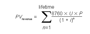
where 
8760 is the number of hours in a year
U is the utilization rate
P is the price per kilowatt⋅hour
i is the interest rate
n is the nth year.

CyclePad calculates the PV of the cost of the cycle in the same manner.  However, figuring the cost of the cycle is a little more involved.  In general, there are two types of cost, fixed and variable.  A fixed cost is only incurred once over the lifetime of the cycle, and is typically incurred in the construction of the cycle.  For example, a turbine might cost $400,000, and if we are an electric utility constructing a new plant, we have to pay General Electric that much money today in order to obtain the turbine.  We might also have to pay a contractor another $75,000 to come in with a crane, lift the turbine into place, and make the necessary connections to enable it to operate.  In the CyclePad economic model, we consider this $75,000 to be a part of the total cost of the turbine, because we incur it once in the course of constructing the power plant, and it is a direct result of our desire to obtain an operating turbine.

These fixed costs are also called capital costs because they are associated with capital assets, such as turbines.  A capital asset is something that persists over time and is used in the process of either making money or obtaining something we value, such as national security.

In contrast, variable costs include the cost of the fuel and maintenance necessary to operate the cycle once it is constructed.  Unlike capital costs, which are independent of whether or not we ever use the cycle, variable costs vary directly with the utilization of the cycle.  For example, utilities construct two types of plants, baseload and peaking.  A baseload plant is expected to run all the time, whereas a peaking plant is only expected to run occasionally, on the hottest and coldest days when the demand for electricity spikes.  Because a baseload plant will incur high variable costs, a key factor in its design will be making it as efficient and robust as possible.  In contrast, since a peaking plant is used infrequently, designers will tend to choose designs that are less expensive to build but more expensive to operate.

The PV of the cycle cost is calculated by assuming that all capital costs are incurred immediately, but variable costs are incurred over the life of the cycle.  To do this calculation, we need to know two things, in addition to the utilization rate, interest rate, and lifetime of the cycle that we needed for the revenue calculation:

•        The total capital cost of the cycle

•        The total annual cost of fuel

•        The total annual maintenance cost

The PV of costs is calculated in a similar manner to the PV for revenue:

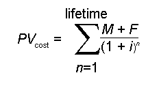
where 
M is the maintenance cost
F is the annual fuel cost
i is the interest rate
n is the nth year.

Each of these costs requires a calculation, so we will discuss them each in turn.

Total Capital Cost

Total capital cost is the sum of the capital cost for each component of the cycle.  However, only the components listed in the following table have a cost model.  Those components lacking a cost model include mixers, splitters, throttles, sources and sinks.  The rationale for this is that these components are little more than conduits (although they can be quite large conduits), and as such are so inexpensive compared to their more complex cousins that their costs would be lost in the noise.

Although one might think that CyclePad could simply apply a cost function to each device and  add up the results, the generality of CyclePad’s device representation requires additional assumptions in the case of heaters and coolers.  In the case of compressors and turbines, it turns out that many designs call for using a set of these devices in series, so each device actually represents a stage of larger device; to obtain accurate costs, we must be sure to apply the cost function only to this larger device, and not to each individual stage.

A heater can (and must) be used to model both the burners in a jet engine, which are little more than cans with holes punched in them to admit atomized fuel, and the boiler of a baseload plant, which in reality might be seven stories tall.  Clearly we cannot capture the cost of each device with one function, so we have added three modeling assumptions for heaters that show up when the control-flag for the economic model is checked.  These assumptions are boiler, burner, and reheater.  A boiler has its own cost function that includes both the capital cost to build and install the device, and the fuel and maintenance costs required to operate it.  To model a reheating vapor cycle, one would use a second heater device to represent the reheater, placing it between two turbines.  In actuality, this reheater is not a separate boiler, but in effect a series of pipes that route the working fluid back through the boiler to reheat it.  The cost function for such a reheater is modeled by applying a reheater-factor to the cost of the boiler in the system.  Consequently, the current CyclePad model is limited to systems containing one boiler, but as such systems comprise the vast majority of vapor power cycles, this limitation should not be too onerous.  Finally, the burner assumption sets the cost of the heater equal to zero, on the basis that the cost is minimal in comparison to the rest of the cycle.  A reheater in a gas cycle (eg, an afterburner for a jet engine) should therefore be modeled as a burner and not a reheater.

In an similar vein, coolers may be used to model both condensers and the atmosphere that, for example, a gas-jet engine exhausts to.  The economic model therefore adds the assumptions condenser and atmosphere to each cooler.  The cost model for a condenser assumes that it is a heat-exchanger whose cold side is a "standard" environment of water from a natural source at 20°C.  No explicit model of additional cooling capital equipment, such as a cooling tower, is included.

There is a related problem one encounters when dealing with turbines and coolers.  In many cases one wants to consider a series of such devices as one aggregate device, as, for example, in a regenerative cycle that bleeds steam from the turbine at several points.  Compressors interleaved with coolers or heat-exchangers represent an intercooled compressor.  CyclePad automatically aggregates compressors and turbines into what we refer to as stage devices, in that they are comprised of a series of stages.  The aggregation is based on an analysis of the structure of the cycle, and only aggregates those devices that do in fact operate in series.  For example, the combined cycle in the Library is comprised of two subcycles communicating via a heat-exchanger.  The top subcycle contains two turbines, which CyclePad identifies as a stage-turbine, and the bottom subcycle contains a lone turbine, which CyclePad identifies as a separate stage turbine of one stage.

The reason for this aggregation is that the cost functions for devices include a factor for estimating the installation cost, and one would not incur a separate installation cost for each stage of a turbine.  The primary complication that stage devices introduce, from the point of view of you, the eternally patient CyclePad user, is that you have to look in the Global Properties menu for the meters that show their properties.  When the economic model is active, however, a message to this effect is posted in each compressor and turbine meter.

The basic equation that CyclePad uses to calculate cost is:

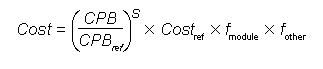
where 
CBP is the cost-basis-parameter
CBPref is the reference cost-basis-parameter
Costref is the reference cost
s is the size-exponent
fmodule is the module factor
fother is the combination of other factors

For example, the cost of a turbine is based on its shaft-power, and the cost of a cooler is based on its area.  CyclePad’s knowledge base contains approximate cost information for each device type, in the form of three parameters, the value of the cost-basis-parameter, the cost of a device operating at that value, and a size-exponent.  For example, a $50,000 pump might require 100kW of input shaft-power to operate.  These two values are plugged into the above equation in order to determine the cost of a different-size pump, say, one that requires 48kW.  The size-exponent governs this relationship.  The data in CyclePad is from Chemical Engineering Economics, (1989) by Donald E. Garrett.

The module factor accounts for the cost of installing the device, and typically falls in a range of 1.2 to 2.0.  The other-factors may include pressure or mass-flow, depending on the device.  For example, the cost of a boiler depends on the mass-flow through the device (this is the cost-basis-parameter), but it also depends on the pressure, since it costs more to build a boiler to withstand higher pressures.  In the table above, the first parameter is the cost-basis-parameter, and any others listed below it are represented as other factors.

Other factors, such as the pressure factor, are calculated as linear functions of the maximum or minimum parameter value the working fluid attains at the inlet or outlet of the device.  These functions were derived from data in Chemical Engineering Economics.

In addition to these factors, a material factor is applied to each device, so one must select a material for each device.  CyclePad contains information on seven materials, including carbon steel, stainless steel, nickel-alloy steel, aluminum, titanium, molybdenum, and unobtainium.  The last is very expensive, but it can withstand extremely high temperatures.  The other six materials have limits on the maximum temperature they can withstand, and CyclePad will signal a contradiction if the temperature of the working fluid flowing through the device is higher than the material’s limit.

Carbon steel is the least expensive material, and is generally well-suited for components that don’t endure particularly high or low temperatures or operate in excessively corrosive environments.  The current CyclePad model does not take corrosive effects into account.

The other materials are superior to carbon steel either in corrosion-resistance, ability to withstand high or low temperatures (e.g., not becoming brittle in a cryogenic cycle), or in density.  Tensile strength is not a concern, as all the materials listed are capable of withstanding the highest pressures attained in thermodynamic cycles.  The material factors for the materials in CyclePad’s knowledge base are relative to carbon steel, which has a factor of 1.0.

Annual Fuel Cost

Heaters that are assumed to be boilers or burners also acquire a fuel property.  CyclePad contains information about the cost per unit-weight and the heating (or calorific) values for five fuels: coal, oil, natural-gas, coal-gas, and hydrogen.  The annual fuel cost for each heater is calculated by the following formula

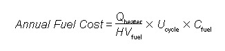
where 
Qheater is the heat output of the heater
HVfuel is the heating value of the fuel
Ucycle is the cycle's utilization rate
Cfuel is the unit costof the fuel

This determines how much fuel is necessary to attain the steady-state heat-flow from the heater to the working fluid and multiplies that amount by the utilizatoin rate of the cycle and the cost per unit weight of the chosen fuel.

Maintenance Cost

Maintenance costs are calculated simply as a fraction of the total capital cost.  Maintenance for a thermodynamic cycle generally falls into the range of 10-20% of the initial capital cost.  If maintenance costs much more than this, say 33%, one would in effect be buying a new cycle every three years or so, and a more robust design that requires less maintenance would be more cost-effective.

Materials Used

CyclePad also contains knowledge about the density of these materials, which it uses to calculate the total weight of the cycle.  CyclePad requires that the control flag Consider Velocity be checked in order to do this calculation, because adding velocity information enables the calculation of cross-sectional area.  The weight calculation is quite abstract, and should not be relied upon to provide accurate estimates of a cycle’s actual weight.  However, it is internally consistent, so it will provide accurate relative measures of the weight of a cycle constructed with two different materials.

The weight function for each device depends on a geometric abstraction of the shape of that device.  For example, the weight function for a turbine models the turbine as a conic section with inlet and outlet diameters derived from the inlet and outlet cross-sectional areas.  The thickness of the conic section is assumed to be 12% of the average outer diameter, and a solid inner cylindrical shaft of 20% of the inlet diameter approximates the weight of the turbine blades.  The weight models for all components are given in the following table

Created with the Personal Edition of HelpNDoc: Generate Kindle eBooks with ease