Investigating a Cycle via the Sensitivity Analysis Tool
To figure out how to improve your design or to more generally explore how changing one parameter affects the value of another, use the sensitivity analysis tool. The form of sensitivity analysis implemented in CyclePad allows you to plot how the value of a dependent parameter changes as the value of an independent parameter varies.
From a design standpoint, the dependent parameter is generally what you would like to improve, such as the thermal efficiency, work produced, or reducing the amount of waste heat. The independent parameter is one of your numerical assumptions whose value affects the dependent parameter, such as the outlet temperature of a boiler or the pressure ratio of a compressor, that you wish to change in order to affect the dependent parameter.
Selecting Sensitivity from the Tools pull-down menu pops-up the Sensitivity Analysis dialog box:
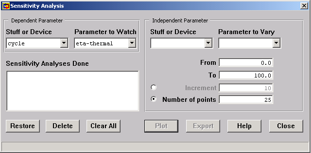
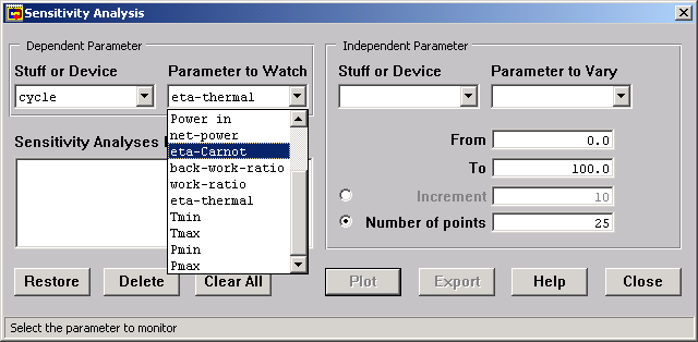
In the upper left of this dialog, you select the parameter of the stuff or device that you would like to watch. By default, this dialog box shows the Cycle as the device and Eta-thermal (the cycle efficiency) as the parameter to affect. Notice that each of the four boxes across the top half of the screen have buttons to their right with arrows pointing down. Clicking on these buttons displays a drop-down menu of the possible choices for that box. In the figure below, you can see that Work Ratio, Eta-Thermal, Min-T, and Max-T (among others) are all possible dependent parameters of the cycle.
In the upper right half of the dialog, you choose the parameter of the stuff or device that you want to vary. These two boxes display only those parameters for which you assumed a value during the analysis phase, because these are the only parameters you can directly vary.
Before you can plot the pressure, you must provide a reasonable range of values for your independent parameter. By default, this range is 0 to 100 in the units of the dependent parameter. You can change it in the lower left part of the screen. The number of points to plot, which defaults to 25, determines the appearance of the resulting graph; more points will make the plot smoother but take more time, particularly if we are using slow but safe sensitivity (see below).
Clicking on the Plot Data button pops up a graph of the behavior of the dependent parameter over the range of the independent parameter:
Moving the mouse pointer over the red points causes the exact x and y values to be displayed in the status bar at the bottom of the screen.
Suppose, for instance, that we wish to examine how the temperature of steam entering the turbine changes the thermal efficiency of a Rankine cycleSimple_Steam_Rankine_Cycle. We set up the following sensitivity analysis.
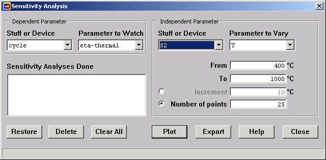
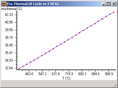
Which produces a plot showing the relation between turbine inlet temperature and the cycle's thermal efficiency.
A concern in performing sensitivity analyses arises in some cycles. CyclePad ordinarily uses an analytical shortcut to speed up the process of generating points for sensitivity analysis plots. The shortcut assumes things like the phase of all the stuffs will stay the same. For certain cycles, this assumption isn't appropriate because, for instance, a state will change from saturated to superheated as we vary the dependent parameter. For such cycles, we must turn on the "Slow But Safe Sensitivity" option under the Preferences | AdvancedPreferences menu item.
For example, consider the same Rankine cycle for which we plotted Thermal Efficiency versus Turbine Inlet Temperature above. Suppose that we were interested in how the thermal efficiency depended on the turbine outlet pressure, which is 100 kPa in the default design and which results in the turbine outlet state being saturated. If we ask CyclePad to plot eta-thermal as P at S3 varies from 50 kPa to 2 MPa, we get the following plot
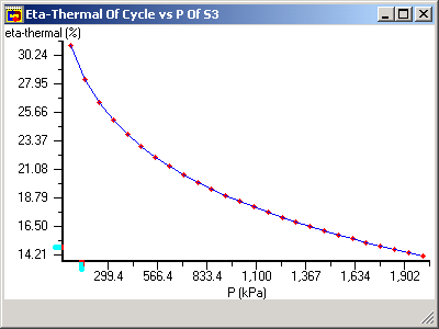
However, since as we raise the outlet pressure the turbine outlet phase eventually becomes a gas. If we turn use slow but safe sensitivity, we get a slightly different outcome.

The difference, though not huge, exists because the slow but safe plot accounts for the transition of the turbine outlet state from saturated to superheated at around 1000 kPa.

Created with the Personal Edition of HelpNDoc: Easily create EPub books