
CyclePad
Design Library
|
CyclePad |
|
Consider an ideal steam cycle in which steam enters the turbine at 5 MPa, 400ºC, and exits at 10 kPa. Calculate the thermal efficiency and the net work per kilogram of steam.
This may not sound like a very complete problem description, since we are given only three numbers. However, it is sufficiently described that we can solve it. Here we will detail the other properties of a Rankine cycle which allow us to complete its design.
The layout shown below is a clickable image. To jump to the part of this page that details the assumptions of a particular device or statepoint, just click on it.
Figure 1: a Rankine cycle |
|
Figure 2: possible heater assumptions
(When we consider non-ideal components, we are often given a pressure loss (or a relation that allows us to compute a pressure loss) for the heater. In that case, we could enter the pressure loss as delta-P for the heater.)
We also notice that we might assume the heater to be isochoric (no change in specific volume or density). Since we will have liquid water entering the heater but steam (which is far less dense) leaving it, we know this is not the likely assumption for an ideal heater.
Looking now at the statepoint after the heater, we know both the pressure and temperature of the fluid at this statepoint from the problem statement. In addition, we are dealing with a steam cycle, so our working fluid is made of water.
We are also given the temperature and pressure at this statepoint. Entering their values, this statepoint's intensive values are completely determined.
When T and P have been entered, CyclePad pauses for a second and figures out the other intensive properties at this statepoint, like specific volume, specific internal energy, et cetera. If we were doing this problem by hand, these are all values we would have to look up in tables.
The next component is the turbine. While we aren't told anything explicitly about this turbine, it is ideal. In general, this means it is isentropic (zero change in entropy) and adiabatic (no heat transfer).
(Even if we did not know that it was ideal, we would probably assume it to be adiabatic because we have not been told how much heat transfer takes place and we have no way to figure it out.)
At the outlet of the turbine, we notice that the specific entropy is already known. (It is the same as that for the statepoint before the turbine because the turbine is isentropic.) We are told in the problem that steam exits at 10 kPa, so we assume the pressure at this statepoint to have that value. Since we now know both the pressure and the entropy at this statepoint, we know all of the intensive property values here. (Once again, CyclePad has saved us much time in table lookup, especially since this statepoint would require interpolation to find.)
We are told the turbine outlet pressure in this problem, and that is the most common case, but there are other possibilities as well. We might instead know:
Note that the turbine outlet quality of 80% is dangerously low for practical use. We might wish to address this problem by adding a reheat stage.
Similar to an ideal heater (and for the same reasons), an ideal cooler has no pressure drop, so we make the isobaric assumption here as we did with HTR1.
Of course, pumps can work with compressed liquids as well, so we could cool the fluid even past saturated fluid down into the compressed liquid region. We do not do this for several reasons related to cycle efficiency.
(Further discussion of pump inlet conditions and their effects on cycle efficiency)
For CyclePad, we can specify that a fluid be saturated by selecting a phase and choosing it to be saturated. Once we have told CyclePad that the phase is saturated, it adds another property to the meter window, allowing us to specify a quality. In this case, we want to assume that quality is zero, since we are forcing the fluid at S4 to be a saturated liquid.
Sometimes we can't cool the working fluid just until it is a saturated liquid. Most often this is because our cooling source is at a specified temperature and we cannot remove the working fluid from the cooler early enough. In these cases, we are usually given a temperature for this state.
We are given no explicit information about the pump, but, like the turbines, ideal pumps are adiabatic and isentropic. We assume both of those things here.
Why does this happen? The reason lays in the approximation that the water in the pump is incompressible, which is very close to accurate, but the slight variation in v between the saturated liquid at the inlet and the compressed liquid at the outlet causes this small heat transfer to show up, confusing CyclePad. This is more likely at low pump inlet pressures (under one atmosphere) than at higher ones.
For our purposes, this heat transfer is not important (it is typically on the order of 0.1% of the work done by the pump), so we can just not worry about whether the pump is adiabatic if some heat transfer has already been found or the adiabatic assumption causes a contradiction.
In general, we might try to change the order in which we make assumptions, just to be certain no contradictions occur later on. We could, for instance, always choose adiabatic before isentropic, or make the pump assumptions before those for the pump inlet. In these instances CyclePad will note the small heat transfer and assume that it is due to round-off accumulation.
Typically, this state is already known because we know the pressure (the same as for the turbine inlet for an isobaric heater) and the entropy (the same as for the pump inlet for an isentropic pump). In cases where this state is not known, it is because we have a non-ideal component in our system (such as a non-isobaric heater). In those cases the problem statement will typically include information about the pump outlet pressure or the pump's pressure ratio.
However, we notice that CyclePad still does not know the many of the values in this cycle. Among the unknown values is the net work per kg of steam and the thermal efficiency, which we are asked to find in the problem statement. The reason is that CyclePad finds some whole cycle properties based on extensive values, which are not known until we assume a mass flow rate (m-dot). (In other words, CyclePad needs the whole heat transfer Q, not the specific heat transfer q).
But a more clever solution is just to assume a mass flow rate so that CyclePad can compute the extensive values it needs to finish the whole cycle calculations. At state S2, we can assume a mass flow rate of 1 kg/sec. Now, we see that those other properties are calculated and, since we have assumed a mass flow of 1 kg/sec, these numbers are per kg of steam.
Download the CyclePad design of the Rankine cycle from here. Whalley, P.B. 1992. Basic Engineering Thermodynamics.
Oxford University Press. ISBN: 0-19-856255-1
Go to
Contributed by: M. E. Brokowski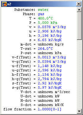
Figure 3: Turbine inlet meter window
The Turbine Inlet (S2)
The Turbine (TUR1)
The Turbine Outlet (S3)
Other Turbine Outlet Assumptions
The Cooler (CLR1)
Figure 4: Preparing the fluid to enter the pump
The Pump Inlet (S4)
This is a statepoint when our own knowledge and reasoning about cycles is key to making assumptions. The only reason we have a cooler before the pump at all is because we know pumps can be damaged by non-liquids. To avoid this, the cooler must condense all of the steam leaving the turbine into a liquid before we send it to the pump. So we at least want to cool our saturated working fluid to 0% quality before sending it to the pump. Figure 4 shows the region to which we must cool the working fluid before safely using a pump.
Other Pump Inlet Assumptions
The Pump (PMP1)
Note
CyclePad uses the equation wpump = -vDP to calculate reversable pump work because the fluid (liquid water) is very close to incompressible. Sometimes CyclePad finds a small heat transfer for the pump and, because this heat transfer isn't quite zero, CyclePad asserts that the pump is not adiabatic or causes a contradiction when we assert that the pump is adiabatic. The Pump Outlet (S1)
Finishing the problem
Our original problem was to find the thermal efficiency of this cycle. Go to the "Cycle" menu and choose "Cycle Properties". This meter window is mostly empty because CyclePad doesn't know which definitions for efficiencies to use and they are different for a heat engine (like our Rankine cycle) than they would be for a refrigeration cycle, for instance. Here we need to tell CyclePad that we are modeling a heat engine. We see that the Carnot efficiency is just over 56.6%.
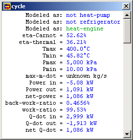
Figure 5: Whole cycle properties
CyclePad Design Files
Related Entries
Sources


or

Initial Entry: 12/1/97
Last Edited: 11/9/01
For comments or suggestions please contact CyclePad-librarian@cs.northwestern.edu